Bill Rankin’s amazing work at Radical Cartography is very inspiring. I’m particularly enamored of his tree maps, both large-scale and small.
I decided to mimic his map of New Haven’s street trees using data for Portland, Oregon, my beautiful town. Sadly, I do not know how he constructed his map at the incredible level of detail it has–I suspect some GIS software I neither have nor know how to use. Instead, I’ll use my trusty hammer: R.
To get the same look as the New Haven map, no existing map package that I’m familiar with would work. I wanted very clean lines, color differentiation for parks and bodies of water, and no labels. To do this, I had to construct the basis for the map from the ground up.
To this end, I downloaded the following:
- The aforementioned Portland street tree inventory
- All roads in Multnomah County
- Bodies of water in Multnomah County
- Parks in the city of Portland
The street trees I cleaned up a little, determining the top 25 genuses and marking all others as “Other.” Any trees missing a trunk diameter got the average for their genus, and all diameters less than 1″ were rounded up to 1. This was done ad-hoc in Excel.
Then, I loaded in my libraries:
[sourcecode language="r"]

library(rgeos)

library(rgdal)

library(plyr)

library(ggplot2)

library(sp)

[/sourcecode]
And my data, which was all normalized to the same projection:
[sourcecode language="r"]

proj <- "+proj=aea +lat_1=45 +lat_2=46 +lon_0=122w +ellps=WGS84"

#--------get tree info-------------

trees <- read.csv("trees.csv", colClasses=c("numeric", "numeric", "character", "character", "numeric", "character", "character", "character"))

coordinates(trees) <- ~ longitude + latitude

proj4string(trees) =CRS("+proj=longlat")

trees <- spTransform(trees, CRS(proj))

trees <- as.data.frame(trees)
#--------------water and parks ----------------
water <- readOGR("C:/Users/Erin/Documents/DataViz/StreetTrees/Water", "tl_2018_41051_areawater")
water <-spTransform(water, CRS(proj))
parks <- readOGR("C:/Users/Erin/Documents/DataViz/StreetTrees/Parks", "Parks_Taxlots")
parks <-spTransform(parks, CRS(proj))
#---------------handle roads-------------------
roads <- readOGR("C:/Users/Erin/Documents/DataViz/StreetTrees/Roads", "tl_2018_41051_roads")
roads <-spTransform(roads, CRS(proj))
majorroads <- subset(roads, MTFCC %in% c("S1100", "S1200"))
minorroads <- subset(roads, !(MTFCC %in% c("S1100", "S1200", "S1630")))
[/sourcecode]
then, a variable to blank out all unnecessary plot stuff
[sourcecode language="r"]blankbg <-theme(axis.line=element_blank(),axis.text.x=element_blank(),

                axis.text.y=element_blank(),axis.ticks=element_blank(),

                axis.title.x=element_blank(), axis.title.y=element_blank(),

                panel.background=element_blank(),panel.border=element_blank(),panel.grid.major=element_blank(),

                panel.grid.minor=element_blank(),plot.background=element_blank())

[/sourcecode]
And one to assign a specific color to each genus. You’ll notice I set TRUE and FALSE to colors as well. This is specifically for when I plot the water shapefile: it’s got islands. TRUE and FALSE map to the “is hole” attribute in the shapefile. If you don’t specify that we want to color holes differently than shapes, the islands will be filled in the same as the rest of the water.
[sourcecode language="r"]plotcolors <- c("TRUE" = "white", "FALSE" = '#E6EFF5', 'Other' = 'white',

                'Acer' = '#ea7058', 'Prunus' = '#ffaaf6', 'Pyrus' = '#f1d6a3', 'Fraxinus' = '#6c8ccc', 'Malus' = '#8bbe42', 'Cornus' = '#872378',

                'Quercus' = '#c6e4be', 'Betula' = '#7ad9ff', 'Tilia' = '#885bd2', 'Crataegus' = '#c43b0b', 'Styrax' = '#ffc094',

                'Liquidambar' = '#9985f2', 'Carpinus' = '#41a7d9', 'Magnolia' = '#3833b8', 'Pinus' = '#96c1ad', 'Ulmuys' = '#1fc154',

                'Pseudotsuga' = '#29654b', 'Juglans' = '#c19e86', 'Parrotia' = '#ffa900', 'Ginkgo' = '#ffe015', 'Zelkova' = '#f75bdf',

                'Nyssa' = '#006eff', 'Thuja' = '#2c835b', 'Cercidiphyllum' = '#f8dbeb', 'Chamaecyparis' = '#4a6895')

[/sourcecode]
Now for the final plot. This took quite a lot of finagling to get just right. For some reason, setting legend.position=”none” inside blankbg just didn’t work, but calling it out specifically did. No clue why. Annoying, but I rolled with it.
[sourcecode language="r"]ggplot()  + coord_equal(xlim = c(-65000, -37000),ylim = c(4690000, 4712500)) +  theme(legend.position="none") + blankbg +

  geom_polygon(data=parks, aes(long, lat, group = group), size = 0.7, fill = '#DCE6C3', alpha = 1)  +

  geom_polygon(data=water, aes(long, lat, group = group, fill = hole), colour = '#cecece', size = .1) +

  geom_path(data = minorroads, mapping = aes(long, lat, group = group), color = "#eaeaea", size = .3) +

  geom_path(data = majorroads, mapping = aes(long, lat, group = group), color = "#eaeaea", size = .8) +

  geom_point(aes(x = longitude, y = latitude, fill = PlotGenus), data = trees, shape = 21, size = trees$DBH/20, alpha = 1,  stroke=.25, color = "#cecece") +

    scale_fill_manual(values = plotcolors, guide = FALSE)[/sourcecode]
I exported it as an ultra-huge SVG to get the smoothest looking result.
[sourcecode language="r"]ggsave("trees.svg", width = 36, height = 29)[/sourcecode]
This I converted to a PNG with Inkscape, and took into Photoshop to add legends and clean up a few wonky lines.
I made a couple different versions. One that looks good on screen. (Fullsize)
And one that looks better printed. My big plan was to get this printed as a wall map, but to get proper detail it’d be huge and prohibitively expensive.
Instead, I mapped out individual neighborhoods in a format that would look good printed at 11×17. This took a bit of research to figure out.
First, I downloaded additional data:
1. outlines of Portland’s neighborhoods
2. all building footprints in Portland
Then I imported them as before. The buildings shapefile is huge and takes a good long time to import.[sourcecode language="r"]
#---------------buildings-----------------
buildings <- readOGR("C:/Users/Erin/Documents/DataViz/StreetTrees/Building", "Building_Footprints")
buildings <-spTransform(buildings, CRS(proj))
#--------------neighborhoods--------------
nhoods <- readOGR("C:/Users/Erin/Documents/DataViz/StreetTrees/Neighborhoods", "Neighborhoods_Regions")
nhoods <-spTransform(nhoods, CRS(proj))
[/sourcecode]
The next step was to clip the roads, parks, and water to the outline of a neighborhood of interest.
[sourcecode language="r"]

nhood <- 'MONTAVILLA'

my_nhood <- subset(nhoods, NAME == nhood)
parks_clip <- raster::intersect(my_nhood, parks)
majorroads_clip <- raster::intersect(majorroads, my_nhood)
minorroads_clip <- raster::intersect(minorroads, my_nhood)
buildings_clip <- raster::intersect(buildings, my_nhood)[/sourcecode]
The tree data includes the neighborhood each tree is in. I decided to rely on this instead of trying to clip the points. I don’t know how precisely how accurate it is, but the outputs look visually pleasing. The tree neighborhoods are sometimes formatted a little differently than the neighbhorhood boundary names, so I use a second nhood variable here.
[sourcecode language="r"]

nhoodtrees <- 'MONTAVILLA'

trees_clip <- subset(trees, Neighborhood == nhoodtrees)[/sourcecode]
Then, to put it all together. Many neighborhoods don’t intersect with the water shapefile, so I commented it out here. I also stacked the roads on top of each other at varying colors to mimic the look of road width.
[sourcecode language="r"]

ggplot()  + coord_equal() +      theme(legend.position="none") + blankbg +

  geom_polygon(data=parks_clip, aes(long, lat, group = group), size = 0.7, fill = '#DCE6C3', alpha = 1)  +

  #geom_polygon(data=water_clip, aes(long, lat, group = group, fill = hole), colour = '#cecece', size = .1) +

  geom_path(data = minorroads_clip, mapping = aes(long, lat, group = group), color = "#eaeaea", size = 1.2) +

  geom_path(data = minorroads_clip, mapping = aes(long, lat, group = group), color = "#ffffff", size = .6) +

  geom_path(data = majorroads_clip, mapping = aes(long, lat, group = group), color = "#eaeaea", size = 2) +

  geom_path(data = majorroads_clip, mapping = aes(long, lat, group = group), color = "#ffffff", size = 1) +

  geom_polygon(data=buildings_clip, aes(long, lat, group = group), size = 0.7, fill = '#f4f4f4', alpha = 1)  +

  geom_point(aes(x = longitude, y = latitude, fill = PlotGenus), data = trees_clip, shape = 21, size =trees_clip$DBH/7, alpha = 1,  stroke=.25, color = "#cecece") +

  scale_fill_manual(values = plotcolors, guide = FALSE)[/sourcecode]
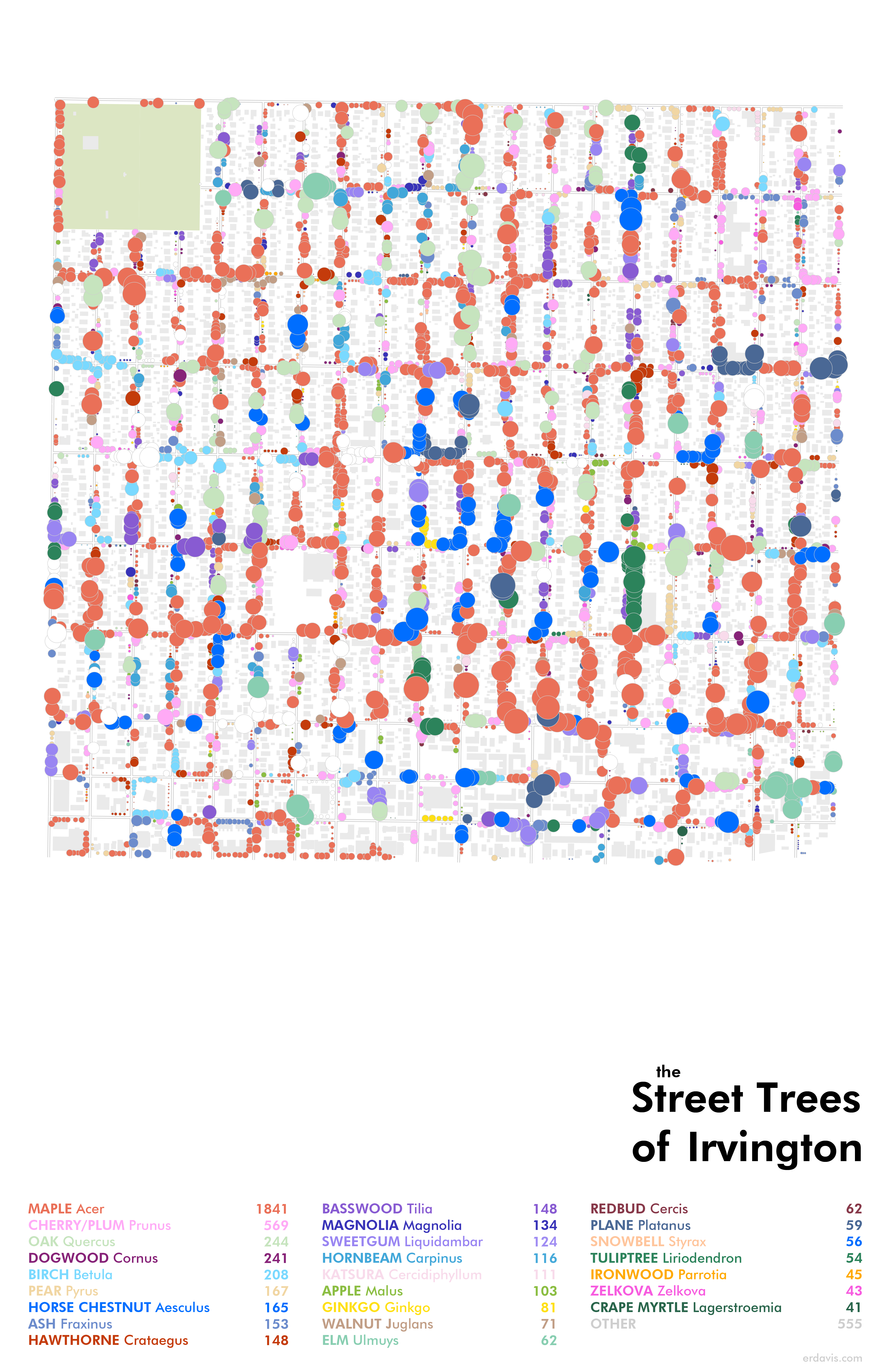
I ultimately do like the results but I’m unsure of some of the details. In particular, I’ve struggled to strike a balance when sizing the tree circles: they need to be large enough to read the color, but small enough not to obscure everything around them. I realized I made a mistake in scaling the circles by diameter instead of by area, but at this point I’m ready to pack it in and call this a post. Before making any prints to hang on the wall, I may go back and fix this.
Discover more from Data Stuff
Subscribe to get the latest posts sent to your email.